R/Finance 2024
Abstract
Implied shocks are a valuable tool for scenario analysis and often used to assess the impact of a change in a variable on a portfolio. For example, a change in the yield curve can be used to assess the impact on a fixed-income portfolio; however, the specification of shocks poses challenges and requires an understanding of the methodology too. In this research paper, we propose an approach to address these challenges by using principal component analysis (PCA) to compute the implied shocks. This paper also presents a methodology to resolve issues related to time-series of eigenanalysis. The utilization of PCA aims to facilitate a more accessible framework for scenario analysis and to deepen the understanding of dynamics driving the scenarios. The numerical calculations use RcppParallel to parallelize rolling eigenanalysis of time-series data, which are available in the rolleigen package on GitHub: https://github.com/jasonjfoster/rolleigen.
Implied shocks
We illustrate an application of implied shocks in scenario analysis using factors X1, Y1, Y2, and Y3.
A single (or subset of) factor(s) is used to specify shocks and then shocks are implied across the other factors for the given scenario. Next the specified and implied shocks are applied to assess the impact on a portfolio. Implied shocks are computed using the following methodology:
beta = (XT X)-1 XT Y
beta <- solve(crossprod(x)) %*% crossprod(x, y)

implied_shocks <- shocks %*% beta
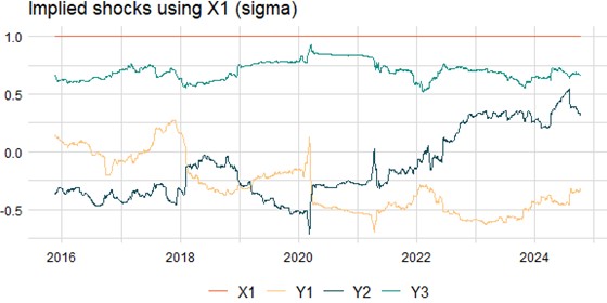
For example, consider the scenario for specifying the X1 factor up one standard deviation:

Data source: the Federal Reserve Economic Data (FRED): https://fred.stlouisfed.org/
roll::roll_crossprod(x, y = NULL, width)
Specifying a single (or subset of) factor(s) for computing implied shocks presents a challenge though. Particularly the specified factor(s) determines both the direction and magnitude of the implied shocks by using the correlation matrix. That is, the direction of the implied shocks is determined by its correlation with only the specified factor(s). Also the variance explained by the specified shock dampens implied shocks on a sigma-adjusted basis by definition. For example, to illustrate the impact of specifying the X1 factor on a sigma-adjusted basis:

Data source: the Federal Reserve Economic Data (FRED): https://fred.stlouisfed.org/
roll::roll_sd(x, width)
To summarize these challenges, the direction of the implied factors is determined and dampened by the specified factor(s). While it is possible to specify all of the shocks to its respective sigma, the direction of the shocks presents yet another challenge. Using the correlation matrix for guidance is an option but the selection of the appropriate row and column is subjective. Instead we propose utilizing PCA to identify the direction and magnitude of the shocks that explain most of the variation in the correlation matrix.
Variance explained
PCA is a dimension reduction technique used to decrease the dimensionality of the data but retain as much information as possible. Essentially, principal components are computed to capture the maximum variance present in the data. The first principal component explains the highest variability, the second principal component (orthogonal to the first) accounts for the second most variability, and so on. The proportion of variance explained by the first i principal components is an indicator for the number of components required to reduce the data’s dimension. This calculation is performed using the eigenvalues of the correlation matrix as follows:

LV <- eigen(cov(x))
L <- LV[["values"]]

variance_explained <- cumsum(L) / sum(L)

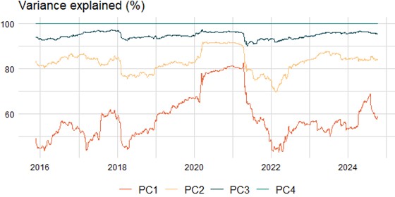
Data source: the Federal Reserve Economic Data (FRED): https://fred.stlouisfed.org/
rolleigen::roll_eigen(x, width)$values
The variance explained by the interquartile range of the first principal component is 52% to 63%. This gives us confidence the first principal component explains most of the variation in the correlation matrix and can be used to identify the direction and magnitude of the shocks. Specifically, the product of the first eigenvector and square root of the first eigenvalue:

LV <- eigen(cov(x))
L <- LV[["values"]]
V <- LV[["vectors"]]

implied_shocks <- sqrt(L[comp]) * V[ , comp]

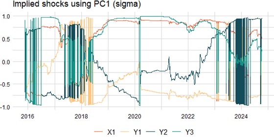
Data source: the Federal Reserve Economic Data (FRED): https://fred.stlouisfed.org/
rolleigen::roll_eigen(x, width)$vectors
As illustrated above, we need to resolve issues related to time-series of eigenanalysis such as flipping the sign and reordering accordingly. These challenges arise given each window is independent of the previous window and floating-point arithmetic is used to calculate the principal components. To address these issues, we can use cosine similarity to match the eigenvectors.
Cosine similarity
Cosine similarity measures the angle between two vectors in a multidimensional space. The cosine of 0° is 1, and it is less than 1 for any other angle; therefore, the cosine similarity between two vectors is 1 if the vectors point in the same direction and 0 if the vectors are orthogonal. The cosine similarity between the eigenvectors of the current window and the previous window is calculated as follows:

LV <- eigen(cov(x))
V <- LV[["vectors"]]

cosine_similarity <- crossprod(V, V0) / sqrt(crossprod(V) * crossprod(V0))
Note: given the eigenvector is already scaled, we can ignore the denominator.
The eigenvector with the highest cosine similarity is selected and sign is multiplied by  to ensure the eigenvector is pointing in the same direction, if needed. The eigenvalues are then reordered accordingly too.

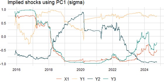
Data source: the Federal Reserve Economic Data (FRED): https://fred.stlouisfed.org/
rolleigen::roll_eigen(x, width, order = TRUE) # default
Now we have addressed the challenges of specified shocks by using PCA to derive implied shocks. That is, we removed the need to select a single (or subset of) factor(s) for computing implied shocks and selected the direction and magnitude of the shocks that explain most of the variation in the correlation matrix. After the sign is adjusted and eigenvalues are reordered, the implied shocks can be used in time-series analysis as well. As illustrated above, each of the sigma-adjusted implied shocks can be less than one during historical periods too.
Conclusion
This research paper introduced an approach to implied shocks that used PCA to address challenges associated with specified shocks. The methodology not only offered a more accessible framework for scenario analysis but also enhanced the understanding of dynamics driving the scenarios. By using PCA to derive implied shocks, and resolving issues related to time-series of eigenanalysis, the methodology both simplified and improved the construction of scenarios. The methodology presented can provide valuable insights for risk managers seeking to refine implied shocks and make more informed decisions on scenario analysis. For more on eigenanalysis, go to https://jasonjfoster.github.io/posts/eigen-r/ for R code and https://jasonjfoster.github.io/posts/eigen-py/ for Python code.
Disclosure: Interactive Brokers
Information posted on IBKR Campus that is provided by third-parties does NOT constitute a recommendation that you should contract for the services of that third party. Third-party participants who contribute to IBKR Campus are independent of Interactive Brokers and Interactive Brokers does not make any representations or warranties concerning the services offered, their past or future performance, or the accuracy of the information provided by the third party. Past performance is no guarantee of future results.
This material is from Jason Foster and is being posted with its permission. The views expressed in this material are solely those of the author and/or Jason Foster and Interactive Brokers is not endorsing or recommending any investment or trading discussed in the material. This material is not and should not be construed as an offer to buy or sell any security. It should not be construed as research or investment advice or a recommendation to buy, sell or hold any security or commodity. This material does not and is not intended to take into account the particular financial conditions, investment objectives or requirements of individual customers. Before acting on this material, you should consider whether it is suitable for your particular circumstances and, as necessary, seek professional advice.


Join The Conversation
If you have a general question, it may already be covered in our FAQs. If you have an account-specific question or concern, please reach out to Client Services.